Search quantum information protocols with LOCCNet
Table of Contents
[1]:
import time
import torch
import math
import numpy as np
import matplotlib.pyplot as plt

import quairkit as qkit
from quairkit import to_state
from quairkit.application import OneWayLOCCNet
from quairkit.database import *
from quairkit.loss import *
from quairkit.operator import *
from quairkit.qinfo import *

qkit.set_dtype('complex128')

plt.rcParams['mathtext.fontset'] = 'cm'
plt.rcParams['font.family'] = 'STIXGeneral'
Introduction
This tutorial explores the application of LOCCNet (Local Operations and Classical Communication Network) in quantum information protocols, particularly in the context of distributed quantum information processing. We will focus on two fundamental tasks[1]:
Quantum State Discrimination: Distinguishing between different quantum states under the restriction of LOCC, specifically discriminating between a perfect Bell state and its noisy counterpart after passing through amplitude damping channels.
Quantum State Distillation: Purifying entangled states to obtain higher-fidelity entanglement using LOCC operations.
Throughout this tutorial, we will demonstrate the practical steps for implementing these protocols. This includes setting up a OneWayLOCCNet for multiple parties, configuring the initial quantum states, and building the parameterized quantum circuits. We will also cover the implementation of parameterized LOCC operations, the visualization of the resulting circuits, and the methods for training and optimizing the network.
Quantum State Discrimination
Problem Description
As demonstrated in [1], distinguishing multipartite quantum states under the restriction of local operations and classical communication (LOCC) is both practically important and theoretically challenging. In particular, the authors focus on discriminating between a perfect Bell state and its noisy counterpart after each qubit has passed through an amplitude damping channel.
Here, to explore the power of LOCCNet in state discrimination, we consider the two ideal Bell states:
and an amplitude damping channel \(\mathcal{A}\) with noise parameter \(\gamma\), defined by:
where the Kraus operators are:
Sending each qubit of \(|\Phi^{-}\rangle\) through \(\mathcal{A}\) yields the mixed state:
while:
remains noiseless. The goal is to distinguish between \(\Phi_0\) and \(\Phi_1\) via LOCC.
The ansatz used for finding QSD protocols with LOCCNet works as follows: the input state is randomly chosen from the set \(\{ \Phi_0, \Phi_1 \}\) with equal probability. Alice performs a unitary gate on her qubit and measures. Then Bob performs on his qubit a unitary gate chosen based on Alice’s measurement result. Bob’s measurement outcome is supposed to tell which state the input state is.
Implementation with LOCCNet
Now we create the OneWayLOCCNet structure. We have two spatially separated parties:
Alice: Has 1 qubit, implements local operations, and performs the first measurement
Bob: Has 1 qubit and performs adaptive operations based on Alice’s measurement
The protocol works as follows:
Alice applies a parameterized unitary gate on her qubit
Alice measures her qubit
Bob receives the classical measurement result
Bob applies a conditional parameterized unitary based on Alice’s outcome
[2]:
def create_locc_network() -> OneWayLOCCNet:
    r"""
    Create a one-way LOCC qubit-network for quantum state discrimination.

    Returns:
        An initialized LOCC network
    """
    party_info = {'Alice': 1, 'Bob': 1}
    net = OneWayLOCCNet(party_info)

    net['Alice'].u3([0])
    net.param_locc(u3, 3, [('Alice', 0),('Bob', 0)], label='M', support_batch=False)

    return net
An example circuit diagram is shown below:
[3]:
create_locc_network().physical_circuit.plot()
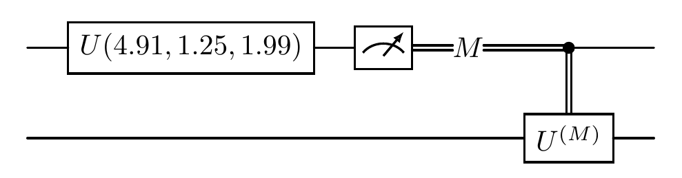
Important Note: In OneWayLOCC, once Alice has measured her first qubit, it cannot be measured again. This restriction ensures we maintain the one-way nature of the classical communication. The following circuit configuration would be forbidden:
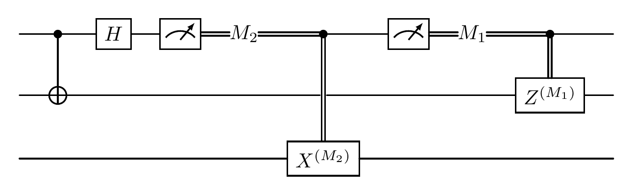
Forbidden Circuit.
Next, we define the quantum states to be discriminated using batch processing:
[4]:
zero2 = torch.tensor([1, 0], dtype=torch.cdouble)
one2 = torch.tensor([0, 1], dtype=torch.cdouble)
basis00 = torch.kron(zero2, zero2)
basis11 = torch.kron(one2, one2)
psi_minus = (basis00 - basis11) / math.sqrt(2)
rho_minus = psi_minus.unsqueeze(1) @ psi_minus.conj().unsqueeze(0)

def generate_single_pair(gamma: float) -> tuple[torch.Tensor, torch.Tensor]:
    r"""
    Generate a pair of quantum states: Bell state and amplitude-damped state.

    Args:
        gamma: Amplitude damping parameter (0 <= gamma <= 1)

    Returns:
        tuple: (Bell state density matrix, amplitude-damped state density matrix)
    """
    state_minus = to_state(rho_minus)
    kraus_ops = amplitude_damping_kraus(gamma)

    state_minus = state_minus.transform(kraus_ops, sys_idx=[0], repr_type="kraus")
    state_minus = state_minus.transform(kraus_ops, sys_idx=[1], repr_type="kraus")

    rho_bell = bell_state(2).density_matrix
    rho_damp = state_minus.density_matrix
    return rho_bell, rho_damp


def generate_initial_states_locc(gamma: float) -> qkit.State:
    r"""Generate batch of initial states for LOCC network training.

    Args:
        gamma: Amplitude damping parameter

    Returns:
        Batch state containing Bell and damped states
    """
    state_bell, state_damp = generate_single_pair(gamma)

    batch = torch.stack([state_bell, state_damp])
    return to_state(batch)
The loss function of this state discrimination protocol is defined as:
where \(P(j\mid \Phi_k)\) is the probability that Bob’s final measurement yields outcome \(j\) given input state \(\Phi_k\). This loss function represents the total error probability in the discrimination task:
\(P(1 \mid \Phi_0)\): Probability of incorrectly identifying the Bell state \(\Phi_0\) as the noisy state
\(P(0 \mid \Phi_1)\): Probability of incorrectly identifying the noisy state \(\Phi_1\) as the Bell state
The implementation works as follows:
Set the initial shared quantum states (\(\Phi_0\) and \(\Phi_1\)) using
net.set_init_state. States that are not set will default to the zero stateExecute the LOCC protocol where Alice measures first
Bob performs conditional operations based on Alice’s outcome
Measure Bob’s qubit to determine the state
Calculate the weighted measurement results across all branches (Alice’s measurement outcomes)
Minimize the loss function to maximize discrimination success probability
We first marginalize the measurement probabilities over all possible branches from Alice’s measurement:
[5]:
def compute_marginalized_probabilities(
    prob_tensor: torch.Tensor, probs_batch: torch.Tensor
) -> torch.Tensor:
    r"""Compute marginalized and normalized measurement probabilities.

    Args:
        prob_tensor: Probability tensor with shape (batch_size, ..., 2)
        probs_batch: Conditional probabilities with same shape structure

    Returns:
        Normalized probabilities with shape (batch_size, 2)
    """
    branch_weights = prob_tensor.sum(dim=2)
    marginalized_probs = torch.einsum('bi,bij->bj', branch_weights, probs_batch)

    norm_sum = marginalized_probs.sum(dim=1, keepdim=True)
    return marginalized_probs / norm_sum
To discriminate between the two quantum states, we classify them based on Bob’s measurement outcome: an outcome of 0 corresponds to the \(\Phi_0\) state (Bell state), and an outcome of 1 corresponds to the \(\Phi_1\) state (damped state).
Our objective is to minimize the loss, which is defined as the average probability of misidentifying the state defined in (6).
[6]:
def compute_discrimination_loss(normalized_probs: torch.Tensor) -> torch.Tensor:
    r"""Compute the average classification probability for state discrimination.

    Based on Bob's measurement outcome: 0 → Bell state, 1 → damped state.
    The function computes the average correct classification probability weighted by
    the prior distribution (0.5 each).

    Args:
        normalized_probs: Shape (2, 2) tensor where normalized_probs[i, j] = P(outcome j | state i)

    Returns:
        Weighted classification score
    """
    p0 = normalized_probs[0].real
    p1 = normalized_probs[1].real

    F0_bell = p0[0]
    T0_bell = p0[1]
    eps = 1e-10
    p0_prob = F0_bell / (F0_bell + T0_bell + eps)

    F1_damped = p1[1]
    T1_damped = p1[0]
    p1_prob = F1_damped / (F1_damped + T1_damped + eps)

    return 0.5 * p0_prob + 0.5 * p1_prob
The main loss function combines the above components:
[7]:
meas = Measure('z')

def loss_func_locc(net: OneWayLOCCNet) -> tuple[torch.Tensor, qkit.State]:
    r"""Compute loss function for LOCC network training.

    Args:
        net: The LOCC network
        inputs: Input states (batch of Bell and damped states)

    Returns:
        tuple: (loss value, output state)
    """
    output_state = net()

    probs_batch, output_state = meas(output_state, qubits_idx=[0], keep_state=True)
    prob_tensor = output_state.probability

    normalized_probs = compute_marginalized_probabilities(prob_tensor, probs_batch)
    return compute_discrimination_loss(normalized_probs)
Now we train the network and analyze how the discrimination success probability varies with the amplitude damping parameter \(\gamma\):
[8]:
def train_locc_network(num_itr: int, lr: float, gamma: float) -> tuple[float, OneWayLOCCNet]:
    r"""
    Train the LOCC network for state discrimination.

    Args:
        num_itr: Number of training iterations
        lr: Learning rate
        gamma: Amplitude damping parameter

    Returns:
        tuple: (best loss value, trained network)
    """
    net = create_locc_network()
    inputs = generate_initial_states_locc(gamma)
    net.set_init_state([('Alice', 0), ('Bob', 0)], inputs)

    time_list = []
    optimizer = torch.optim.Adam(net.parameters(), lr=lr)
    scheduler = torch.optim.lr_scheduler.ReduceLROnPlateau(optimizer, 'min', factor=0.5)

    best_loss = float('inf')
    best_state = None

    for itr in range(num_itr):
        start_time = time.time()
        optimizer.zero_grad()

        loss = loss_func_locc(net)

        loss.backward()
        optimizer.step()

        loss = loss.item()
        scheduler.step(loss)
        time_list.append(time.time() - start_time)

        if loss < best_loss:
            best_loss = loss
            best_state = {k: v.cpu().clone() for k, v in net.state_dict().items()}

        if itr % 100 == 0 or itr == num_itr - 1:
            print(f"iter: {str(itr).zfill(len(str(num_itr)))}, " +
              f"loss: {loss:.4f}, best = {best_loss:.4f}, " +
              f"lr: {scheduler.get_last_lr()[0]:.2E}, avg_time: {np.mean(time_list):.4f}s")

    if best_state:
        net.load_state_dict(best_state)

    return best_loss, net
[9]:
NUM_ITR = 200
LR = 0.15
START_POINT = 0

gamma_vals_full = np.linspace(0.0, 1.0, 11)
gamma_vals = gamma_vals_full[START_POINT:]
results = []

print(f"Training LOCC network for gamma values: {gamma_vals}\n")

for idx, gamma in enumerate(gamma_vals):
    print(f"\nTraining gamma = {gamma:.2f} ({idx+1}/{len(gamma_vals)})")
    best_loss, trained_net = train_locc_network(NUM_ITR, LR, gamma)
    sp = 1 - best_loss
    results.append(sp)
    print(f"Result: success_prob = {sp:.6f}\n")

print("\nFinal Results:")
for gamma, sp in zip(gamma_vals, results):
    print(f"gamma = {gamma:.2f}, success_prob = {sp:.6f}")
Training LOCC network for gamma values: [0.  0.1 0.2 0.3 0.4 0.5 0.6 0.7 0.8 0.9 1. ]


Training gamma = 0.00 (1/11)
iter: 000, loss: 0.6240, best = 0.6240, lr: 1.50E-01, avg_time: 0.0940s
iter: 100, loss: 0.0000, best = 0.0000, lr: 1.50E-01, avg_time: 0.0048s
iter: 199, loss: 0.0000, best = 0.0000, lr: 3.75E-02, avg_time: 0.0041s
Result: success_prob = 1.000000


Training gamma = 0.10 (2/11)
iter: 000, loss: 0.7643, best = 0.7643, lr: 1.50E-01, avg_time: 0.0050s
iter: 100, loss: 0.0244, best = 0.0244, lr: 7.50E-02, avg_time: 0.0040s
iter: 199, loss: 0.0243, best = 0.0243, lr: 2.93E-04, avg_time: 0.0038s
Result: success_prob = 0.975657


Training gamma = 0.20 (3/11)
iter: 000, loss: 0.4448, best = 0.4448, lr: 1.50E-01, avg_time: 0.0034s
iter: 100, loss: 0.0472, best = 0.0472, lr: 9.37E-03, avg_time: 0.0034s
iter: 199, loss: 0.0472, best = 0.0472, lr: 3.66E-05, avg_time: 0.0035s
Result: success_prob = 0.952769


Training gamma = 0.30 (4/11)
iter: 000, loss: 0.4493, best = 0.4493, lr: 1.50E-01, avg_time: 0.0073s
iter: 100, loss: 0.0684, best = 0.0684, lr: 4.69E-03, avg_time: 0.0037s
iter: 199, loss: 0.0684, best = 0.0684, lr: 9.16E-06, avg_time: 0.0041s
Result: success_prob = 0.931564


Training gamma = 0.40 (5/11)
iter: 000, loss: 0.4977, best = 0.4977, lr: 1.50E-01, avg_time: 0.0046s
iter: 100, loss: 0.0877, best = 0.0877, lr: 1.87E-02, avg_time: 0.0040s
iter: 199, loss: 0.0877, best = 0.0877, lr: 3.66E-05, avg_time: 0.0040s
Result: success_prob = 0.912310


Training gamma = 0.50 (6/11)
iter: 000, loss: 0.5179, best = 0.5179, lr: 1.50E-01, avg_time: 0.0067s
iter: 100, loss: 0.1047, best = 0.1047, lr: 3.75E-02, avg_time: 0.0041s
iter: 199, loss: 0.1047, best = 0.1047, lr: 7.32E-05, avg_time: 0.0038s
Result: success_prob = 0.895285


Training gamma = 0.60 (7/11)
iter: 000, loss: 0.3539, best = 0.3539, lr: 1.50E-01, avg_time: 0.0056s
iter: 100, loss: 0.1192, best = 0.1192, lr: 7.50E-02, avg_time: 0.0043s
iter: 199, loss: 0.1192, best = 0.1192, lr: 2.93E-04, avg_time: 0.0040s
Result: success_prob = 0.880789


Training gamma = 0.70 (8/11)
iter: 000, loss: 0.3938, best = 0.3938, lr: 1.50E-01, avg_time: 0.0071s
iter: 100, loss: 0.1309, best = 0.1309, lr: 7.50E-02, avg_time: 0.0039s
iter: 199, loss: 0.1309, best = 0.1309, lr: 2.93E-04, avg_time: 0.0042s
Result: success_prob = 0.869121


Training gamma = 0.80 (9/11)
iter: 000, loss: 0.3783, best = 0.3783, lr: 1.50E-01, avg_time: 0.0122s
iter: 100, loss: 0.1394, best = 0.1394, lr: 9.37E-03, avg_time: 0.0040s
iter: 199, loss: 0.1394, best = 0.1394, lr: 1.83E-05, avg_time: 0.0040s
Result: success_prob = 0.860555


Training gamma = 0.90 (10/11)
iter: 000, loss: 0.5038, best = 0.5038, lr: 1.50E-01, avg_time: 0.0037s
iter: 100, loss: 0.1447, best = 0.1447, lr: 9.37E-03, avg_time: 0.0034s
iter: 199, loss: 0.1447, best = 0.1447, lr: 1.83E-05, avg_time: 0.0034s
Result: success_prob = 0.855316


Training gamma = 1.00 (11/11)
iter: 000, loss: 0.3794, best = 0.3794, lr: 1.50E-01, avg_time: 0.0121s
iter: 100, loss: 0.1464, best = 0.1464, lr: 3.75E-02, avg_time: 0.0052s
iter: 199, loss: 0.1464, best = 0.1464, lr: 7.32E-05, avg_time: 0.0050s
Result: success_prob = 0.853553


Final Results:
gamma = 0.00, success_prob = 1.000000
gamma = 0.10, success_prob = 0.975657
gamma = 0.20, success_prob = 0.952769
gamma = 0.30, success_prob = 0.931564
gamma = 0.40, success_prob = 0.912310
gamma = 0.50, success_prob = 0.895285
gamma = 0.60, success_prob = 0.880789
gamma = 0.70, success_prob = 0.869121
gamma = 0.80, success_prob = 0.860555
gamma = 0.90, success_prob = 0.855316
gamma = 1.00, success_prob = 0.853553
[10]:
plt.figure(figsize=(6, 4))
plt.plot(gamma_vals, results, marker='o')
plt.xlabel(r'$\gamma$')
plt.ylabel('Success Probability (1 - loss)')
plt.title(f'Success Probability vs AD channel parameter $\\gamma$ (LOCCNet)')
plt.grid(True)
plt.show()
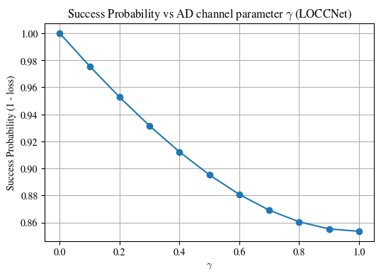
As shown in the figure above, as the noise parameter \(\gamma\) increases, the success probability of distinguishing between the two states \(\Phi_0\) and \(\Phi_1\) decreases, indicating that they become harder to distinguish.
Quantum State Distillation
Problem Setup
Bell state distillation (also known as entanglement distillation) is a crucial task in quantum information processing. The goal is to extract high-fidelity entangled pairs from a larger number of noisy entangled pairs using only LOCC operations.
In this task, Alice and Bob share 4 noisy Bell states and they apply local operations and measurements to distill fewer but higher-quality entangled pairs, using a combination of single-qubit variational gates and CNOT gates.
Implementation
Our implementation uses OneWayLOCCNet with the following structure:
Alice and Bob: Each has 4 qubits
Circuit architecture: Two layers of single-qubit variational gates sandwich a layer of cycled CNOT gates
Optimization goal: Maximize the fidelity of the distilled entangled pairs
[11]:
net_purify = OneWayLOCCNet({'Alice': 4, 'Bob': 4})

net_purify['Alice'].u3([0, 1, 2, 3])
net_purify['Alice'].cnot('cycle')
net_purify['Alice'].u3([0, 1, 2, 3])

net_purify['Bob'].u3([0, 1, 2, 3])
net_purify['Bob'].cnot('cycle')
net_purify['Bob'].u3([0, 1, 2, 3])
Purification Protocol Details
The states we want to purify are S states, which are probabilistic mixtures of Bell states and \(|00\rangle\) states:
The protocol works as follows:
Use
net.set_init_stateto set the initial state for each pair of qubits shared between Alice and BobMeasure all qubits except the first qubit of Alice and Bob
Compare measurement results for the three qubit pairs (pairs 1, 2, and 3). We consider the distillation successful if, for each of these three pairs, Alice’s measurement outcome is the same as Bob’s (e.g., \(m_{A_1} = m_{B_1}\), \(m_{A_2} = m_{B_2}\), and \(m_{A_3} = m_{B_3}\)). If the measurement outcome is not in this list, the protocol fails for this round, and the pair is discarded.
If the measurement outcomes for any pair do not match, the protocol fails for this round, and the pair is discarded.
If successful, use partial trace to discard the measured states (pairs 1, 2, and 3).
The remaining state (on the first pair of qubits, pair 0) is the distilled state.
Our loss function is \(1 - F\), where \(F\) is the state fidelity between the distilled state (after partial trace) and the target EPR state \(|\Phi^{+}\rangle = \frac{|00\rangle + |11\rangle}{\sqrt{2}}\).
[12]:
meas = Measure('zzzzzz')
target_state = bell_state(2)

measurement_qubits = [1, 5, 2, 6, 3, 7]
successful_outcomes = [
    '000000', '000011', '001100', '110000',
    '001111', '111100', '110011', '111111'
]

def purify(net: OneWayLOCCNet, share_entangle: bool) -> torch.Tensor:
    r""" Perform entanglement purification protocol.

    Args:
        net: The purification LOCC network
        share_entangle: Whether share entangled pairs initially
    """

    net._state_map.clear()

    if share_entangle:
        for i in range(4):
            net.set_init_state([('Alice', i), ('Bob', i)])

    status = net()
    _, post_state = meas(status, qubits_idx=measurement_qubits,
                         desired_result=successful_outcomes, keep_state=True)

    reduced_state = post_state.trace(measurement_qubits)
    return 1 - state_fidelity(reduced_state, target_state).mean()
Now we define the S state parameter \(p = 0.7\) and begin training:
[13]:
NUM_ITR = 100
LR = 0.2

p = 0.7
[14]:
time_list = []
opt = torch.optim.Adam(net_purify.parameters(), lr=LR)
scheduler = torch.optim.lr_scheduler.ReduceLROnPlateau(opt, 'min', factor=0.5)

for itr in range(NUM_ITR):
    start_time = time.time()
    opt.zero_grad()

    loss_bell = purify(net_purify, share_entangle=True)
    loss_00 = purify(net_purify, share_entangle=False)

    loss = p * loss_bell + (1-p) * loss_00

    loss.backward()
    opt.step()

    loss = loss.item()
    scheduler.step(loss)
    time_list.append(time.time() - start_time)

    if itr % 20 == 0 or itr == NUM_ITR - 1:
        print(f"iter: {str(itr).zfill(len(str(NUM_ITR)))}, " +
              f"loss: {loss:.4f}, " +
              f"lr: {scheduler.get_last_lr()[0]:.2E}, avg_time: {np.mean(time_list):.4f}s")

final_loss_bell = purify(net_purify, share_entangle=True)
final_loss_00 = purify(net_purify, share_entangle=False)
final_loss = p * final_loss_bell + (1-p) * final_loss_00

final_fidelity = 1 - final_loss.item()
print(f"\nTraining Complete! Final Fidelity: {final_fidelity:.5f}")
iter: 000, loss: 0.6801, lr: 2.00E-01, avg_time: 0.0599s
iter: 020, loss: 0.1106, lr: 2.00E-01, avg_time: 0.1583s
iter: 040, loss: 0.0902, lr: 2.00E-01, avg_time: 0.1046s
iter: 060, loss: 0.0882, lr: 2.00E-01, avg_time: 0.0835s
iter: 080, loss: 0.0879, lr: 2.00E-01, avg_time: 0.0741s
iter: 099, loss: 0.0879, lr: 1.00E-01, avg_time: 0.0668s

Training Complete! Final Fidelity: 0.91213
We first establish the baseline fidelity by calculating the fidelity between the initial S state \(\rho_s\) and the target Bell state \(\rho_{target} = |\Phi^+\rangle\langle\Phi^+|\).
The fidelity formula for a mixed state \(\rho_s\) and a pure target state \(\rho_{target}\) simplifies to:
This calculation yields the simplified formula:
For our initial state with \(p=0.7\), the baseline fidelity is:
Our resulting distilled fidelity of 0.9212 is higher than this 0.85 baseline, demonstrating that the LOCCNet protocol successfully purified the entanglement.
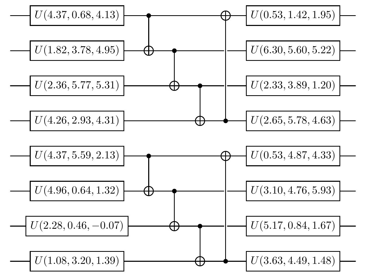
The experimental circuit diagram is shown below:
[15]:
net_purify.physical_circuit.plot()
References
[1] Zhao, Xuanqiang, et al. “Practical distributed quantum information processing with LOCCNet.” npj Quantum Information 7.1 (2021): 159.
Notation Reference
Table: A reference of notation conventions in this tutorial.
Symbol |
Variant |
Description |
|---|---|---|
\(\|\Phi^{+}\rangle\) |
Bell state (maximally entangled) |
|
\(\|\Phi^{-}\rangle\) |
Bell state with phase flip |
|
\(\|00\rangle\) |
Product state of two qubits in zero state |
|
\(\mathcal{A}\) |
Amplitude damping channel |
|
\(\gamma\) |
Noise parameter for amplitude damping |
|
\(E_0, E_1\) |
Kraus operators for the amplitude damping channel |
|
\(\rho\) |
Density matrix |
|
\(\Phi_0\) |
Noiseless Bell state (to be discriminated) |
|
\(\Phi_1\) |
Noisy state after amplitude damping (to be discriminated) |
|
\(L\) |
Loss function |
|
\(P(j\|\Phi_k)\) |
Conditional probability of outcome \(j\) given state \(\Phi_k\) |
|
\(\rho_s\) |
S state (mixed state for purification) |
|
\(p\) |
Mixing parameter in S state |
|
\(F\) |
State fidelity |
[16]:
qkit.print_info()
---------VERSION---------
quairkit: 0.5.1
torch: 2.11.0+cu130
torch cuda: 13.0
numpy: 2.2.6
scipy: 1.15.3
matplotlib: 3.10.5
---------SYSTEM---------
Python version: 3.10.18
OS: Linux
OS version: #1 SMP PREEMPT_DYNAMIC Thu Jun  5 18:30:46 UTC 2025
---------DEVICE---------
CPU:  13th Gen Intel(R) Core(TM) i9-13980HX
GPU: (0) NVIDIA GeForce RTX 4090 Laptop GPU