[ ]:

%%bash
if ! python -c "import quairkit" 2>/dev/null; then
    pip install -i https://mirrors.tuna.tsinghua.edu.cn/pypi/web/simple quairkit
fi

if ! command -v pdftotext &> /dev/null; then
    conda install -y -c conda-forge poppler
fi

Entanglement¶

Copyright (c) 2025 QuAIR team. All Rights Reserved.

In this tutorial, we explore the fascinating phenomenon of quantum entanglement, a fundamental and non-classical feature of quantum mechanics that underlies many modern quantum technologies. We begin by introducing the historical background of entanglement, including its emergence from the Einstein-Podolsky-Rosen (EPR) paradox and its formalization through Bell’s theorem. We then provide a mathematical description of entangled states and discuss their physical significance. Additionally, we demonstrate how to use QuAIRKit to simulate measurement statistics that violate classical bounds.

Table of Contents

• Introduction

  • Background

• Bell’s Inequality

  • Definition

  • Classical Theory

  • Quantum Entanglement

    • Tensor Product of Hilbert Spaces

    • Separable vs. Entangled States

  • Quantum Prediction of Bells Inequality

• Bell’s Experiment with QuAIRKit

  • State preparation

  • Sampling experiment

• Other Types of Entangled States

  • GHZ State

  • W State

• Discussion

[2]:

import torch

import quairkit as qkit
from quairkit import Circuit, Hamiltonian

Introduction¶

Background¶

The journey into the world of quantum entanglement began in the early 20th century, as quantum mechanics was first being formulated to describe the strange behavior of matter and energy at the atomic and subatomic scales. In 1935, Albert Einstein, Boris Podolsky, and Nathan Rosen (EPR) introduced a thought experiment that challenged the then-accepted understanding of quantum theory [1-2]. Their paper highlighted a phenomenon, which Schrödinger would later call “entanglement,” where two particles could be linked in such a way that measuring a property of one instantaneously influences the other, regardless of the distance separating them. This “spooky action at a distance,” as Einstein famously called it, seemed to violate the principles of local realism and suggested that quantum mechanics was an incomplete theory.

For decades, the EPR paradox remained largely a philosophical debate. It wasn’t until 1964 that physicist John Stewart Bell developed a mathematical framework, now known as Bell’s theorem, that transformed the debate into a testable hypothesis [3]. Bell’s theorem demonstrated that no physical theory based on local realism could ever reproduce all of the predictions of quantum mechanics. This paved the way for experimental verification. Starting in the 1970s and culminating in the definitive experiments by Alain Aspect in the early 1980s, physicists were able to conclusively demonstrate that the predictions of quantum mechanics were correct and that the universe does indeed permit these strange, non-local correlations. These experiments confirmed the reality of entanglement, cementing its status as one of the most profound and foundational, yet persistently mysterious, features of the quantum world.

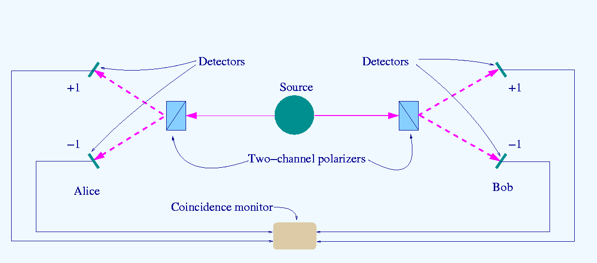
Figure 1. Schematic of the Bell test experiments by Alain Aspect’s team between 1980 and 1982. Its 1982 result offered an experimental answer to the EPR paradox.

This diagram illustrates a detailed setup of the Aspect experiment, a landmark test of Bell’s inequality. A source at the center emits entangled photon pairs in opposite directions, toward two observers—Alice and Bob. Each photon passes through a two-channel polarizer, whose orientation can be rapidly switched during the photon’s flight. Depending on the polarizer angle, the photon is directed toward one of two detectors, registering a result of either +1 or −1. A coincidence monitor records the joint outcomes of both sides. Crucially, the ability to randomly and quickly vary the polarizer settings ensures that the measurement choices are space-like separated, ruling out local hidden variable explanations. The correlations measured between Alice and Bob’s outcomes violate Bell’s inequality, confirming the nonlocal nature of quantum entanglement.

Alain Aspect, John Clauser, and Anton Zeilinger were honored the 2022 Nobel Prize in Physics for their pioneering work on experimental tests of Bell’s inequality.

Bell’s Inequality¶

Definition¶

Bell’s theorem provides a mathematical framework to test whether the universe s based on local realism or quantum mechanics. It sets an upper limit on how strongly correlated the measurements on two separated particles can be, assuming that their properties are predetermined and that no influence can travel faster than light. Quantum mechanics, however, predicts that entangled particles can exhibit stronger correlations than this classical limit allows.

John Bell’s original 1964 inequality was formulated based on perfect correlations. A common expression derived from his work, considering measurements along three different axes (\(a, b, c\)), can be written in terms of the probabilities of getting different outcomes:

This form, however, relies on ideal conditions that are difficult to achieve. A more experimentally robust version was developed in 1969, known as the CHSH inequality. Instead of probabilities, it uses a correlation value, \(S\), derived from four separate measurements. The CHSH inequality is given by:

Here, \(a\) and \(a'\) are two different measurement settings for the first particle (e.g., two angles of a polarizer), and \(b\) and \(b'\) are two settings for the second particle. The term \(E(a, b)\) is the statistical correlation of the outcomes when the settings \(a\) and \(b\) are used. Quantum mechanics predicts that for specific choices of measurement settings on an entangled pair, the value of \(|S|\) can be as high as

thus violating the classical limit.

Classical Theory¶

The classical derivation of Bell’s inequality can be broken down into two common-sense ideas:

1. Realism: Physical properties of objects exist independently of whether they are being measured. For two separated particles, the outcome of any potential measurement is predetermined by a set of “hidden variables” (often denoted by \(\lambda\)). These variables contain all the information about the particle pair.

2. Locality: The result of a measurement performed at one location cannot be instantaneously influenced by events at a distant location. In other words, information cannot travel faster than the speed of light. The measurement outcome for Alice’s particle depends only on her detector setting and the hidden variables, not on Bob’s setting.

Let’s use this framework to derive the CHSH inequality. We’ll denote the outcome of Alice’s measurement with setting \(a\) as \(A(a, \lambda)\) and Bob’s with setting \(b\) as \(B(b, \lambda)\) which outcome can only take one of two values: +1 or -1.

The CHSH expression, for a single particle pair determined by \(\lambda\), is:

Now, let’s consider the values for Bob’s predetermined outcomes, \(B(b, \lambda)\) and \(B(b', \lambda)\). Since they must be either +1 or -1, there are two possibilities:

• Case 1: \(B(b, \lambda) = B(b', \lambda)\). Then:

  \[B(b, \lambda) + B(b', \lambda) = \pm 2, \quad B(b, \lambda) - B(b', \lambda) = 0, \tag{4}\]
  \[S(\lambda) = A(a, \lambda)(\pm 2) + A(a', \lambda)(0) = \pm 2, \tag{5}\]

• Case 2: \(B(b, \lambda) = -B(b', \lambda)\). Then:

  \[B(b, \lambda) + B(b', \lambda) = 0, \quad B(b, \lambda) - B(b', \lambda) = \pm 2, \tag{6}\]
  \[S(\lambda) = A(a, \lambda)(0) + A(a', \lambda)(\pm 2) = \pm 2, \tag{7}\]

In either case, \(S(\lambda) \in \{-2, +2\}\). Therefore, for any hidden variable \(\lambda\):

To obtain the experimentally measurable quantity, we average over many runs:

Since the average of bounded values \(\pm 2\) cannot exceed 2 in magnitude, we obtain the classical bound:

Any physical theory based on hidden variables must obey this inequality. Therefore, if an experiment shows a result where \(|S| > 2\), it directly refutes the principle of local realism.

Quantum Entanglement¶

Before we explore how quantum mechanics violates Bell’s inequality, we must understand why such a violation is even possible. The key lies in the unique mathematical structure of entangled states, which exhibit correlations beyond what any classical theory can predict.

To explain entanglement rigorously, we begin by introducing the concept of tensor product—the mathematical foundation for describing joint quantum systems.

Tensor Product of Hilbert Spaces¶

We have already known that in quantum mechanics, the state of a system is represented by a unit vector in a complex Hilbert space. For a single qubit, the Hilbert space is \(\mathcal{H} = \mathbb{C}^2\), with basis states denoted as \(|0\rangle = \begin{pmatrix}1 \ 0\end{pmatrix}\) and \(|1\rangle = \begin{pmatrix}0 \ 1\end{pmatrix}\).

For a composite system of two qubits (two subsystems \(A\) and \(B\)), the joint system is represented in the tensor product space: \(\mathcal{H}_{AB} = \mathcal{H}_A \otimes \mathcal{H}_B\). If \(|\psi\rangle \in \mathcal{H}_A\) and \(|\phi\rangle \in \mathcal{H}_B\), then their combined state is:

This operation satisfies bilinearity:

The standard computational basis for two qubits is:

Separable vs. Entangled States¶

A separable (product) state is a state in \(\mathcal{H}_A \otimes \mathcal{H}_B\) that can be written as:

Such states describe two subsystems that are independent, in the sense that the measurement outcome on one has no influence on the other. Even when described by a mixed density matrix \(\rho_{AB}\), a state is called separable if it can be expressed as:

By contrast, a pure state is entangled if it cannot be factored into a product of local states. The canonical examples of entangled states are the Bell states, such as:

These states cannot be written as any product of individual qubit states.

While separable states produce correlations that obey Bell’s inequality and can be explained by local hidden variables, entangled states can generate much stronger correlations that violate this classical limit. These nonlocal correlations arise not from any signal, but from a shared quantum state that remains connected regardless of distance. This inseparable nature is precisely what allows quantum theory to make predictions impossible under classical physics.

Quantum Prediction of Bell’s Inequality¶

We now turn to quantum mechanics to understand how and why it predicts a violation of Bell’s inequality. Unlike classical physics, measurement outcomes in quantum mechanics are not predetermined but are defined only at the moment of observation. To illustrate this, consider the following Bell state,

Here, \(|0\rangle\) and \(|1\rangle\) are the eigenstates of the Pauli-Z matrix: \(\sigma_z\), which represents a measurement of the qubit’s spin along the Z-axis.

In this scenario, one qubit is sent to Alice and the other to Bob. Their measurement choices are defined as specific physical observables, represented by different Pauli matrices.

Alice chooses to measure one of two observables:

• \(a = \sigma_z\) (measurement along the Z-axis)

• \(a' = \sigma_x = \begin{pmatrix} 0 & 1 \\ 1 & 0 \end{pmatrix}\) (measurement along the X-axis)

Bob chooses to measure one of his two observables:

• \(b = -\frac{\sigma_x + \sigma_z}{\sqrt{2}}\) (measurement along a diagonal axis between the -X and -Z directions)

• \(b' = \frac{\sigma_x - \sigma_z}{\sqrt{2}}\) (measurement along a diagonal axis between the +X and -Z directions)

In quantum mechanics, the expected correlation between Alice’s and Bob’s measurements is calculated using the Born rule: \(E(a, b) = \langle\psi| a \otimes b |\psi\rangle\). Although the calculation involves matrix algebra, the results for the four possible pairs of measurements are given as:

• \(\langle a \otimes b \rangle = \frac{1}{\sqrt{2}}\)

• \(\langle a \otimes b' \rangle = \frac{1}{\sqrt{2}}\)

• \(\langle a' \otimes b \rangle = \frac{1}{\sqrt{2}}\)

• \(\langle a' \otimes b' \rangle = -\frac{1}{\sqrt{2}}\)

Now we can compute the value for a specific combination of these correlations, as defined in the CHSH inequality test:

This value is significantly greater than the classical limit of 2!

This theoretical result demonstrates that quantum mechanics is fundamentally incompatible with local realism. When a measurement is made on one entangled particle, the shared quantum state of the system is updated instantly, influencing the outcome of the other particle. It shows that the “spooky action at a distance” is not a sign of an incomplete theory, but rather a sign that the universe possesses a profound, non-local connectedness.

Bell’s experiment with QuAIRKit¶

In this section, we demonstrate how to numerically verify the CHSH inequality using QuAIRKit. To this end, we must prepare a pair of entangled qubits, send them to two distant measurement stations, and measure each qubit using one of two possible settings. For each pair of settings \((a, b)\), \((a, b')\), \((a', b)\), and \((a', b')\), the measurement outcomes are collected and the correlation values \(E(a, b)\), etc., are computed.

State preparation¶

First, we need to prepare the two-qubit entangled state that Alice and Bob will share. We will construct the Bell state \(\ket{\Psi^-}\).

[3]:

# Construct a circuit to generate the Bell state |Ψ⁻⟩
num_qubits = 2
bell_circuit = Circuit(num_qubits)
bell_circuit.h(0)
bell_circuit.cx([0, 1])
bell_circuit.x(1)
bell_circuit.z(1)

# Get the final state vector
bell_state = bell_circuit()

print("Bell State |Ψ⁻⟩ prepared:")
print(bell_state.ket)

Bell State |Ψ⁻⟩ prepared:
tensor([[ 0.0000+0.j],
        [-0.7071+0.j],
        [ 0.7071+0.j],
        [ 0.0000+0.j]])

We can define the local observables for Alice and Bob. Each observable is represented as a Hamiltonian object acting on either qubit 0 (Alice) or qubit 1 (Bob). These operators correspond to the measurement settings used in the CHSH inequality test.

[4]:

inv_sqrt_2 = 1 / torch.sqrt(torch.tensor(2.0))


# Alice's observables (acting on qubit 0)
A0 = Hamiltonian([[1.0, "Z0,I1"]])
A1 = Hamiltonian([[1.0, "X0,I1"]])

# Bob's observables (acting on qubit 1)
B0 = Hamiltonian([
    [-inv_sqrt_2, "I0,X1"],
    [-inv_sqrt_2, "I0,Z1"]
])
B1 = Hamiltonian([
    [inv_sqrt_2, "I0,X1"],
    [-inv_sqrt_2, "I0,Z1"]
])

print(f"Hamiltonian for Alice's observable A0:\n{A0}")
print(f"\nHamiltonian for Bob's observable B0:\n{B0}")

Hamiltonian for Alice's observable A0:
1.0 Z0, I1

Hamiltonian for Bob's observable B0:
-0.7071067690849304 I0, X1
-0.7071067690849304 I0, Z1

The joint observables are constructed by combining Alice’s and Bob’s local observables into two-qubit Hamiltonians acting on both qubits.

[5]:

# a ⊗ b = Z ⊗ (−X − Z)/√2
A0B0 = Hamiltonian([
    [-inv_sqrt_2, "Z0,X1"],
    [-inv_sqrt_2, "Z0,Z1"]
])

# a ⊗ b' = Z ⊗ (X − Z)/√2
A0B1 = Hamiltonian([
    [inv_sqrt_2, "Z0,X1"],
    [-inv_sqrt_2, "Z0,Z1"]
])

# a' ⊗ b = X ⊗ (−X − Z)/√2
A1B0 = Hamiltonian([
    [-inv_sqrt_2, "X0,X1"],
    [-inv_sqrt_2, "X0,Z1"]
])

# a' ⊗ b' = X ⊗ (X − Z)/√2
A1B1 = Hamiltonian([
    [inv_sqrt_2, "X0,X1"],
    [-inv_sqrt_2, "X0,Z1"]
])

Sampling experiment¶

We now compute the expectation values of the four terms in the CHSH expression using QuAIRKit’s expec_val() function. If the resulting \(|S|\) exceeds 2, the simulation confirms a violation of the classical CHSH inequality, in agreement with quantum mechanical predictions.

[6]:

# Calculate the expectation value for each setting using the prepared Bell state
e00 = bell_state.expec_val(A0B0)
e01 = bell_state.expec_val(A0B1)
e10 = bell_state.expec_val(A1B0)
e11 = bell_state.expec_val(A1B1)

# Calculate the final CHSH value
S = e00 + e01 + e10 - e11

print(f"Expectation value <A0 B0>: {e00.item():.4f}")
print(f"Expectation value <A0 B1>: {e01.item():.4f}")
print(f"Expectation value <A1 B0>: {e10.item():.4f}")
print(f"Expectation value <A1 B1>: {e11.item():.4f}")
print("-" * 30)
print(f"Simulated CHSH value S = {S.item():.4f}")

# Verify the violation
if abs(S.item()) > 2:
    print("\nCHSH inequality violated! (|S| > 2)")
else:
    print("\nCHSH inequality not violated. (|S| <= 2)")

Expectation value <A0 B0>: 0.7071
Expectation value <A0 B1>: 0.7071
Expectation value <A1 B0>: 0.7071
Expectation value <A1 B1>: -0.7071
------------------------------
Simulated CHSH value S = 2.8284

CHSH inequality violated! (|S| > 2)

Other Types of Entangled States¶

While Bell states are the simplest examples of quantum entanglement between two qubits, quantum systems with three or more qubits reveal richer entanglement structures. Two of the most well-known genuinely entangled three-qubit states are the GHZ state and the W state.

GHZ State¶

The Greenberger-Horne-Zeilinger (GHZ) state for three qubits is defined as:

This state is maximally entangled in the sense that measurement on any one qubit collapses the entire system. However, it is fragile: if any one qubit is lost or traced out, the remaining two are left in a separable state.

W State¶

The W state for three qubits is defined as:

Unlike the GHZ state, the W state is robust to particle loss: if one qubit is lost, the remaining two qubits are still entangled.

GHZ and W states are not convertible into one another via local operations and classical communication (LOCC), indicating that they belong to inequivalent classes of multipartite entanglement. Understanding their properties is crucial in the study of quantum foundations, quantum secret sharing, and distributed quantum computing.

Discussion¶

Quantum entanglement represents one of the most profound departures of quantum mechanics from classical intuition. It describes a non-classical correlation between subsystems that persists regardless of spatial separation, and has been experimentally verified through violations of Bell inequalities. As such, entanglement is not only a theoretical curiosity but also a fundamental physical resource.

In modern quantum technologies, entanglement plays a central role. It powers quantum teleportation, superdense coding, and quantum key distribution (QKD) in quantum communication. In quantum computing, entangled states form the backbone of quantum speedup, enabling algorithms such as Shor’s and Grover’s to outperform their classical counterparts. In quantum sensing, quantum metrology leverages entangled states to achieve measurement precision beyond classical limits. Future research aims to develop more robust entanglement generation schemes, entanglement witnesses, and fault-tolerant architectures that can harness large-scale multipartite entanglement for scalable quantum computation and secure global quantum networks.

References¶

[1] Skibba, Ramin. “Einstein, Bohr and the war over quantum theory.” Nature 555.7698 (2018).

[2] Einstein, Albert, Boris Podolsky, and Nathan Rosen. “Can quantum-mechanical description of physical reality be considered complete?.” Physical Review 47.10 (1935): 777.

[3] Bell, John S. “On the Einstein-Podolsky-Rosen paradox.” Physics 1.3 (1964): 195.

Table: A reference of notation conventions in this tutorial.

[7]:

qkit.print_info()

---------VERSION---------
quairkit: 0.4.2
torch: 2.8.0+cu128
torch cuda: 12.8
numpy: 2.2.6
scipy: 1.15.3
matplotlib: 3.10.6
---------SYSTEM---------
Python version: 3.10.18
OS: Linux
OS version: #1 SMP Tue Nov 5 00:21:55 UTC 2024
---------DEVICE---------
CPU:  13th Gen Intel(R) Core(TM) i9-13980HX
GPU: (0) NVIDIA GeForce RTX 4090 Laptop GPU